UE Bistatic Sensing

UE bistatic sensing observes the same $h_\mathrm{DL}(t,\tau)$ as downlink communication, but communication removes the channel while sensing preserves its frequency-domain and slow-time-domain structure. The UE must reconstruct unknown data symbols and prevent BS–UE timing drift from moving the sensing delay axis.

1. Downlink-Symbol Reconstruction

ZC, pilot, and full-band channel-reference symbols are known. On data resources, the UE directly hard-decides the equalized QPSK symbols to reduce sensing-reconstruction complexity and latency, without LDPC re-encoding or constellation remapping:

$$\tilde b_{n,m,\gamma}^\mathrm{DL} =\frac{1}{\sqrt2} \left[ \operatorname{sgn}(\operatorname{Re}\{\hat d_{n,m,\gamma}^\mathrm{DL}\}) +j\operatorname{sgn}(\operatorname{Im}\{\hat d_{n,m,\gamma}^\mathrm{DL}\}) \right].$$

The unified reconstructed grid is

$$\tilde b_{n,m,\gamma}= \begin{cases} b_{n,m,\gamma}^\mathrm{DL},&(n,m)\in\Omega_\mathrm{ref}^\mathrm{DL} \text{ or }m\in\mathcal S_\mathrm{ZC}^\mathrm{DL},\\ \tilde b_{n,m,\gamma}^\mathrm{DL},&(n,m)\in\Omega_\mathrm{data}^\mathrm{DL}. \end{cases}$$

Removing communication modulation gives

$$F_{n,m,\gamma}^\mathrm{UE} =\frac{Y_{n,m,\gamma}^\mathrm{DL}} {\tilde b_{n,m,\gamma}}.$$

Correct decisions make $F_{n,m,\gamma}^\mathrm{UE}$ a time-frequency sample of the BS-to-UE channel. Decision errors create sparse outliers, so low-SNR sensing may select only high-confidence data or known references.

2. Why Communication Timing Is Insufficient

Communication only needs the total delay spread to remain within the cyclic prefix. Sub-sample timing offset may remain in the phase of $\hat H_{n,m,\gamma}^\mathrm{DL}$; the downlink demodulation boundary moves only when accumulated drift approaches the threshold.

Bistatic sensing measures delay itself. Reusing these discrete corrections creates staircase delay trajectories and artificial discontinuities in delay-Doppler and micro-Doppler results. Sensing therefore needs a continuous timing estimate that accounts for every integer jump of the communication frame origin.

OpenISAC provides two alternative bistatic-timing methods: OTA LoS tracking, which uses only the downlink observation, and eRTM, which uses both uplink and downlink channels. The two methods do not simultaneously drive the sensing timing correction for the same frame.

Alternative Bistatic Timing Options

OTA LoS Tracking Option

OTA LoS tracking uses only the UE downlink estimate and continuously tracks the LoS-path coordinate relative to the current downlink demodulation boundary. From the Signal Model, this coordinate is

$$\tau_\mathrm{LoS}^\mathrm{UE}(t) =\tau_{\mathrm{LoS,prop}}(t) +\tau_\mathrm{TO}^\mathrm{UE}(t).$$

The downlink demodulation-window position is represented by $\tau_d^\mathrm{UE}$ and is included in the UE timing offset $\tau_\mathrm{TO}^\mathrm{UE}$ through

$$\tau_\mathrm{TO}^\mathrm{UE} =\tau_\mathrm{DL}^\mathrm{RF}-\tau_d^\mathrm{UE}.$$

From the synchronization-ZC channel estimate,

$$p_\gamma[k] =\frac{1}{N}\sum_{n=0}^{N-1} \hat H_{n,m_\mathrm{sync},\gamma}^\mathrm{DL} e^{j2\pi nk/N}.$$

For integer peak $k_{\max,\gamma}$, define

$$r_\gamma[q] =\frac{p_\gamma[k_{\max,\gamma}+q]} {p_\gamma[k_{\max,\gamma}]}, \qquad q\in\{-1,1\}.$$

The Quinn-type fractional candidates are

$$\hat\delta_{\tau,+} =\frac{r_\gamma[1]}{r_\gamma[1]-1}, \qquad \hat\delta_{\tau,-} =\frac{r_\gamma[-1]}{1-r_\gamma[-1]}.$$

After selecting $\hat\delta_{\tau,\gamma}$ by candidate-sign consistency, the current LoS observed-coordinate estimate is

$$\hat k_{\tau,\gamma} =k_{\max,\gamma}+\hat\delta_{\tau,\gamma}, \qquad \hat\tau_{o,\gamma}=\frac{\hat k_{\tau,\gamma}}{B}.$$

For a window of $\Gamma_W$ frames beginning at $\gamma_w$, let $\hat k_\mathrm{TO,\gamma}$ be the integer timing correction already applied by communication. Its cumulative coordinate change is

$$A_{\gamma_w+\ell} =\sum_{i=0}^{\ell-1}\hat k_\mathrm{TO,\gamma_w+i}, \qquad \ell=0,\ldots,\Gamma_W-1,$$

and the continuous observations are

$$\tilde k_{\tau,\gamma_w+\ell} =\hat k_{\tau,\gamma_w+\ell}+A_{\gamma_w+\ell}.$$

Fit the slowly varying sampling-clock drift with

$$\tilde k_{\tau,\gamma_w+\ell} \approx \epsilon_\mathrm{SIO,w}\ell+k_{\tau,\gamma_w}, \qquad \epsilon_\mathrm{SIO,w}=MN_sB\,\Delta T_{as,w}.$$

The continuous sensing timing recursion is

$$\hat k_{\tau,\gamma}^\mathrm{sens} =\hat k_{\tau,\gamma-1}^\mathrm{sens} +\hat\epsilon_\mathrm{SIO,w-1} -\hat k_\mathrm{TO,\gamma-1} +\mu_\gamma e_\gamma,$$ $$e_\gamma =\hat k_{\tau,\gamma} -\hat k_{\tau,\gamma-1}^\mathrm{sens}.$$

The prediction advances the trajectory, the integer-correction term preserves its coordinate, and the feedback term limits accumulated model error. The frequency-domain correction is

$$\tilde F_{n,m,\gamma}^\mathrm{UE} =F_{n,m,\gamma}^\mathrm{UE} \exp\!\left\{ j2\pi\kappa_n\Delta f \left( \frac{\hat k_{\tau,\gamma}^\mathrm{sens}}{B} +mN_s\Delta\hat T_{as,w-1} \right) \right\}.$$

This option removes both the true LoS propagation delay and the UE TO, so the output delay is referenced to the LoS path. It requires LoS to remain visible; if LoS disappears or the dominant peak switches, the tracked coordinate no longer represents the same physical path.

eRTM Bidirectional Timing Option [1]

Delay and Timing-Offset Relationship

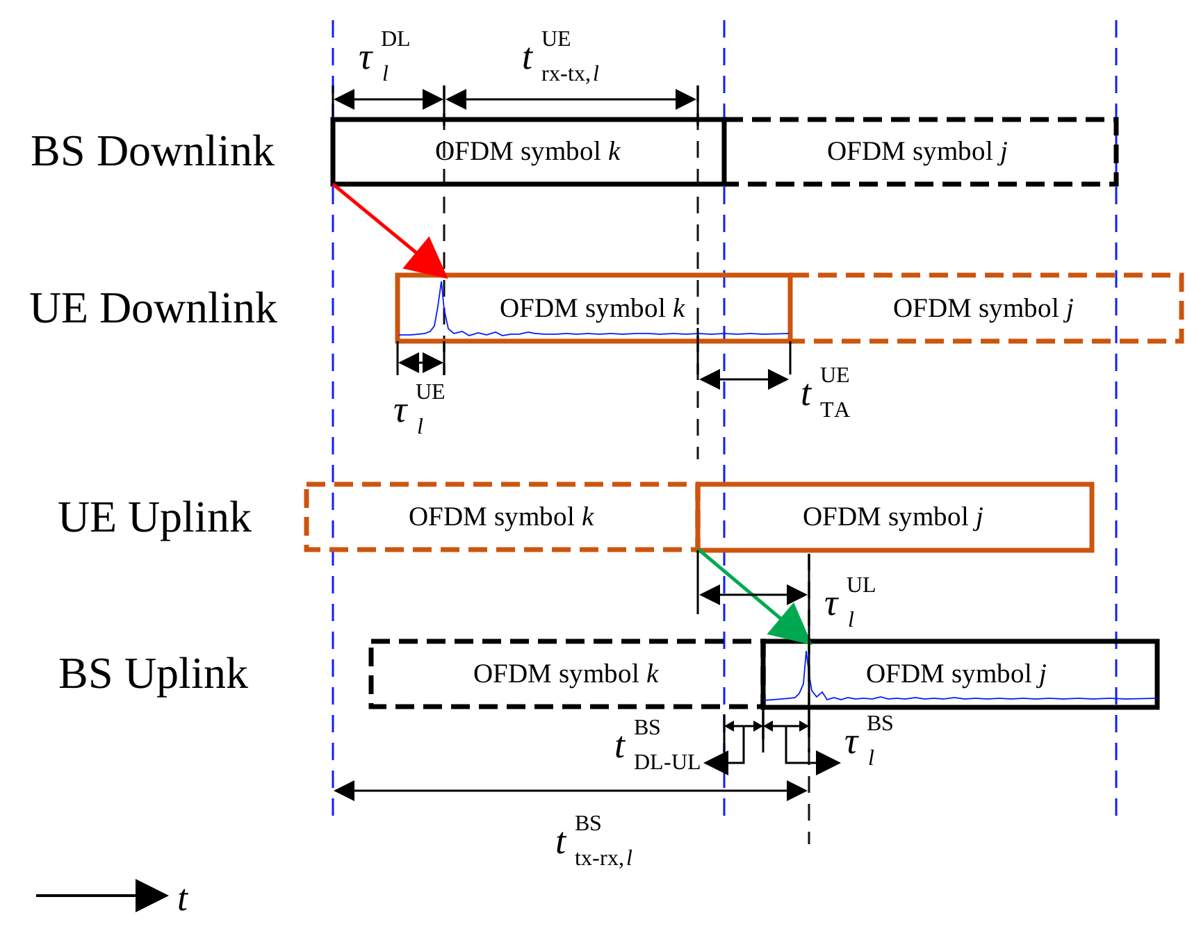
The diagram shows the relationship among the downlink reference signal, its corresponding uplink reference signal, propagation delays, timing advance, and the delays observed at the two endpoints.

For the same downlink/uplink reference-boundary pair, assume that $T$ is the theoretical time difference between the downlink reference signal and its corresponding uplink reference signal on the OFDM grid. Let $t_\mathrm{DL-UL}^\mathrm{BS}$ be the BS downlink-transmit/uplink-receive reference-boundary difference and $t_\mathrm{TA}^\mathrm{UE}$ the UE uplink timing advance. With the UE downlink reference boundary as time zero, downlink path $l$ arrives at $\tau_l^\mathrm{UE}$ and the uplink is transmitted at $T-t_\mathrm{TA}^\mathrm{UE}$, so

$$t_{\mathrm{rx-tx},l}^\mathrm{UE} =T-\tau_l^\mathrm{UE}-t_\mathrm{TA}^\mathrm{UE}.$$

With the BS downlink reference boundary as time zero, the BS uplink-receive reference boundary is at $T+t_\mathrm{DL-UL}^\mathrm{BS}$ and uplink path $l$ is delayed from it by $\tau_l^\mathrm{BS}$, so

$$t_{\mathrm{tx-rx},l}^\mathrm{BS} =T+\tau_l^\mathrm{BS}+t_\mathrm{DL-UL}^\mathrm{BS}.$$

Subtracting the UE receive-to-transmit waiting interval leaves the total downlink and uplink link delay:

$$t_{\mathrm{tx-rx},l}^\mathrm{BS} -t_{\mathrm{rx-tx},l}^\mathrm{UE} =\tau_l^\mathrm{DL}+\tau_l^\mathrm{UL}.$$

Substituting these intervals together with $\tau_l^\mathrm{DL}=\tau_{l,\mathrm{prop}}+\tau_\mathrm{DL}^\mathrm{RF}$ and $\tau_l^\mathrm{UL}=\tau_{l,\mathrm{prop}}+\tau_\mathrm{UL}^\mathrm{RF}$ gives

$$\tau_l^\mathrm{BS}+\tau_l^\mathrm{UE} =2\tau_{l,\mathrm{prop}}+\tau_\mathrm{DL}^\mathrm{RF} +\tau_\mathrm{UL}^\mathrm{RF} -t_\mathrm{DL-UL}^\mathrm{BS} -t_\mathrm{TA}^\mathrm{UE}.$$

Define the path-independent term

$$\tau_c =\tau_\mathrm{DL}^\mathrm{RF} +\tau_\mathrm{UL}^\mathrm{RF} -t_\mathrm{DL-UL}^\mathrm{BS} -t_\mathrm{TA}^\mathrm{UE},$$

The path delays observed at the two endpoints therefore satisfy

$$\boxed{ \tau_l^\mathrm{BS}+\tau_l^\mathrm{UE} =2\tau_{l,\mathrm{prop}}+\tau_c }.$$

Finally, substituting $\tau_l^\mathrm{UE}=\tau_{l,\mathrm{prop}}+\tau_\mathrm{TO}^\mathrm{UE}$ and $\tau_l^\mathrm{BS}=\tau_{l,\mathrm{prop}}+\tau_\mathrm{TO}^\mathrm{BS}$ gives

$$\boxed{ \tau_\mathrm{TO}^\mathrm{BS} +\tau_\mathrm{TO}^\mathrm{UE} =\tau_c }.$$

$\tau_c$ can be calculated directly from system-calibration parameters and known runtime parameters. Specifically, add the calibrated downlink and uplink RF group delays, then subtract the runtime offset between the BS downlink-transmit and uplink-receive reference boundaries and the UE uplink timing advance. The two receivers observe $\tau_l^\mathrm{BS}$ and $\tau_l^\mathrm{UE}$, respectively.

eRTM uses the BS-side uplink estimate $\hat H_{\mathrm{BS}}[n]$ and UE-side downlink estimate $\hat H_{\mathrm{UE}}[n]$ from closely spaced reference symbols. Because TO varies slowly, $\tau_\mathrm{TO}^\mathrm{BS}(t_{\mathrm{UL}})$ and $\tau_\mathrm{TO}^\mathrm{UE}(t_{\mathrm{DL}})$ for the same measurement pair are abbreviated as $\tau_\mathrm{TO}^\mathrm{BS}$ and $\tau_\mathrm{TO}^\mathrm{UE}$. Under the TDD reciprocity conditions, the Signal Model gives

$$H_{\mathrm{BS}}[n] \approx H_{\mathrm{UE}}[n] e^{-j2\pi\kappa_n\Delta f \tau_\mathrm{TO}^{\mathrm{BS-UE}}}.$$

In FDD, eRTM reliability decreases if the visible path sets or path scattering coefficients differ excessively between the two carriers. The first eRTM step estimates the differential TO $\tau_\mathrm{TO}^{\mathrm{BS-UE}}$ using either a frequency-domain maximum-likelihood metric or a delay-magnitude-spectrum metric.

Select the runtime metric with uplink.ertm_timing_metric. delay_magnitude is the default and keeps the existing phase-robust delay-magnitude correlation with centroid3 peak refinement. maximum_likelihood uses the white-noise, unknown-common-phase ML form below and applies three-point parabolic peak refinement. The CPU and CUDA implementations evaluate the ML metric as a complex circular correlation of the two oversampled delay responses; by the correlation theorem, this is equivalent to the frequency-domain $\operatorname{IFFT}\{\hat H_\mathrm{BS}\hat H_\mathrm{UE}^{*}\}$ expression.

Maximum-Likelihood Metric

Let the common unknown channel on the UE’s current delay axis be

$$H_{0,\gamma}[n] =\sum_{l=0}^{L-1}\alpha_l e^{-j2\pi\kappa_n\Delta f [\tau_{l,\mathrm{prop}}+\tau_\mathrm{TO}^\mathrm{UE}]}.$$

Let the quantity to be estimated, $\tau$, represent $\tau_\mathrm{TO}^{\mathrm{BS-UE}}$. The observation model is

$$\hat H_{\mathrm{BS}}[n] =H_{0,\gamma}[n]e^{-j2\pi\kappa_n\Delta f\tau} +V_{\mathrm{BS},\gamma}[n],$$ $$\hat H_{\mathrm{UE}}[n] =H_{0,\gamma}[n]+V_{\mathrm{UE},\gamma}[n],$$ $$V_{\mathrm{BS},\gamma}[n]\sim\mathcal{CN}(0,\sigma_{\mathrm{BS},n}^2), \qquad V_{\mathrm{UE},\gamma}[n]\sim\mathcal{CN}(0,\sigma_{\mathrm{UE},n}^2),$$

with independent endpoint noise. Eliminating the common channel gives

$$\hat\tau_\mathrm{TO}^{\mathrm{BS-UE},\mathrm{ML}} =\arg\min_\tau \sum_{n=0}^{N-1} \frac{ \left| \hat H_{\mathrm{BS}}[n] e^{j2\pi\kappa_n\Delta f\tau} -\hat H_{\mathrm{UE}}[n] \right|^2 }{\sigma_{\mathrm{BS},n}^2+\sigma_{\mathrm{UE},n}^2}.$$

With calibrated common phase, this is equivalent to

$$\hat\tau_\mathrm{TO}^{\mathrm{BS-UE},\mathrm{ML}} =\arg\max_\tau \operatorname{Re}\!\left\{ \sum_{n=0}^{N-1} \frac{ \hat H_{\mathrm{BS}}[n]\hat H_{\mathrm{UE}}^{*}[n] }{\sigma_{\mathrm{BS},n}^2+\sigma_{\mathrm{UE},n}^2} e^{j2\pi\kappa_n\Delta f\tau} \right\}.$$

With unknown common phase, maximize the magnitude instead:

$$\hat\tau_\mathrm{TO}^{\mathrm{BS-UE},\mathrm{ML}} =\arg\max_\tau \left| \sum_{n=0}^{N-1} \frac{ \hat H_{\mathrm{BS}}[n]\hat H_{\mathrm{UE}}^{*}[n] }{\sigma_{\mathrm{BS},n}^2+\sigma_{\mathrm{UE},n}^2} e^{j2\pi\kappa_n\Delta f\tau} \right|.$$

For white noise, the constant denominator may be omitted. On a length-$P$ discrete search grid, define

$$q_\gamma[p] =\operatorname{IFFT}_{P}\!\left\{ \frac{ \hat H_{\mathrm{BS}}[n]\hat H_{\mathrm{UE}}^{*}[n] }{\sigma_{\mathrm{BS},n}^2+\sigma_{\mathrm{UE},n}^2} \right\}.$$

Then

$$\hat p=\arg\max_p|q_\gamma[p]|.$$

Map the circular-IFFT peak index to a signed delay bin:

$$\hat p_\mathrm{s} = \begin{cases} \hat p, &\hat p\le \dfrac{P}{2},\\ \hat p-P, &\hat p>\dfrac{P}{2}. \end{cases}$$

Let $Q[p]=|q_\gamma[p]|$. Using the peak and its two circular neighbors, the three-point parabolic fractional-bin refinement is

$$\hat\delta_p =\frac{1}{2} \frac{ Q[(\hat p-1)\bmod P]-Q[(\hat p+1)\bmod P] }{ Q[(\hat p-1)\bmod P]-2Q[\hat p]+Q[(\hat p+1)\bmod P] }.$$

Then,

$$\hat\tau_\mathrm{TO}^{\mathrm{BS-UE},\mathrm{ML}} =\frac{\hat p_\mathrm{s}+\hat\delta_p}{P\Delta f}.$$

Delay-Magnitude-Spectrum Metric

When the uplink and downlink channels have poor phase consistency because of reference-signal separation, transmit/receive system-response differences, or similar effects, cross-correlating their delay-magnitude spectra reduces sensitivity to the phase mismatch and improves differential-TO robustness.

Let $P=L_\mathrm{os}N$ be the zero-padded IFFT length, with the remaining $P-N$ frequency-domain coefficients set to zero. Using the subcarrier index $\kappa_n$ directly, the oversampled delay response and magnitude are

$$\tilde h_{q,\gamma}[p] =\frac{1}{P} \sum_{n=0}^{N-1} \hat H_{q,\gamma}[\kappa_n] e^{j2\pi\kappa_n p/P}.$$

The corresponding delay-magnitude spectrum is

$$a_{q,\gamma}[p] =|\tilde h_{q,\gamma}[p]|, \qquad p=0,\ldots,P-1, \qquad q\in\{\mathrm{BS},\mathrm{UE}\}.$$

Circularly correlate the two delay-magnitude spectra:

$$C_\mathrm{amp}[d] =\sum_{p=0}^{P-1} a_{\mathrm{BS},\gamma}[p] a_{\mathrm{UE},\gamma}^{\vphantom{*}}[(p-d)\bmod P].$$

Let the circular-correlation peak index be

$$\hat d=\arg\max_d C_\mathrm{amp}[d].$$

Map it to a signed delay bin:

$$\hat d_\mathrm{s} = \begin{cases} \hat d, &\hat d\le \dfrac{P}{2},\\ \hat d-P, &\hat d>\dfrac{P}{2}. \end{cases}$$

Three-point parabolic interpolation gives the fractional-bin refinement

$$\hat\delta_d =\frac{1}{2} \frac{ C_\mathrm{amp}[(\hat d-1)\bmod P] -C_\mathrm{amp}[(\hat d+1)\bmod P] }{ C_\mathrm{amp}[(\hat d-1)\bmod P] -2C_\mathrm{amp}[\hat d] +C_\mathrm{amp}[(\hat d+1)\bmod P] }.$$

Therefore,

$$\hat\tau_\mathrm{TO}^{\mathrm{BS-UE},\mathrm{amp}} =\frac{\hat d_\mathrm{s}+\hat\delta_d}{P\Delta f}.$$

This metric uses the complete multipath delay structure rather than subtracting two dominant peaks.

Separating BS and UE Timing Offsets

The Delay and Timing-Offset Relationship gives:

$$\left\{ \begin{aligned} \tau_\mathrm{TO}^\mathrm{BS} +\tau_\mathrm{TO}^\mathrm{UE} &=\tau_c,\\ \tau_\mathrm{TO}^\mathrm{BS} -\tau_\mathrm{TO}^\mathrm{UE} &=\tau_\mathrm{TO}^{\mathrm{BS-UE}}. \end{aligned} \right.$$

Solving this system gives

$$\left\{ \begin{aligned} \tau_\mathrm{TO}^\mathrm{UE} &=\frac{\tau_c-\tau_\mathrm{TO}^{\mathrm{BS-UE}}}{2},\\ \tau_\mathrm{TO}^\mathrm{BS} &=\frac{\tau_c+\tau_\mathrm{TO}^{\mathrm{BS-UE}}}{2}. \end{aligned} \right.$$

The UE frequency-domain correction is

$$\tilde F_{n,m,\gamma}^\mathrm{UE} =F_{n,m,\gamma}^\mathrm{UE} e^{j2\pi\kappa_n\Delta f \hat\tau_\mathrm{TO}^\mathrm{UE}}.$$

A positive physical delay creates a negative frequency-domain slope, hence the positive compensation exponent.

Bistatic Output and Resolution

Before sensing timing compensation, downlink path $l$ has coordinate

$$\tau_l^\mathrm{UE} =\tau_{l,\mathrm{prop}} +\tau_\mathrm{TO}^\mathrm{UE}$$

relative to the current UE demodulation boundary. OTA LoS tracking compensates the LoS observed coordinate $\tau_{\mathrm{LoS,prop}}+\tau_\mathrm{TO}^\mathrm{UE}$ and therefore reports propagation delay relative to LoS:

$$\tilde\tau_{l,\mathrm{OTA}} =\tau_{l,\mathrm{prop}} -\tau_{\mathrm{LoS,prop}}.$$

eRTM estimates and removes $\tau_\mathrm{TO}^\mathrm{UE}$ separately, preserving the true propagation delay:

$$\tilde\tau_{l,\mathrm{eRTM}} =\tau_l^\mathrm{UE} -\hat\tau_\mathrm{TO}^\mathrm{UE} \approx\tau_{l,\mathrm{prop}}.$$

The corrected $\tilde F_{n,m,\gamma}^\mathrm{UE}$ is concatenated in slow time for clutter rejection, a delay-Doppler 2D FFT, or micro-Doppler processing. With contiguous bandwidth $B=N\Delta f$, delay resolution is $\Delta\tau=1/B$, corresponding to bistatic total-path-length resolution $\Delta d_\mathrm{bi}=c/B$. Uniform frequency sampling has circular delay-ambiguity period $1/\Delta f$, while the interference-free delay spread should remain within $T_\mathrm{CP}$. For slow-time interval $T_\mathrm{slow}$ and coherent length $M_s$, Doppler resolution is $1/(M_sT_\mathrm{slow})$ and the two-sided unambiguous interval is $\pm1/(2T_\mathrm{slow})$.

Applicability

• OTA LoS tracking requires a persistently visible LoS path; LoS loss or reference-peak switching can be mistaken for clock drift.
• eRTM does not require a LoS path, but both directions must be enabled, fixed RF group delays must be calibrated, and the uplink and downlink channels must have sufficiently similar propagation structures.
• TDD best matches the reciprocity model within the coherence time. FDD complex path coefficients are not necessarily reciprocal, so correlation is approximate and depends on corresponding principal path delays; if the visible path sets or path scattering coefficients differ too much between the two carriers, eRTM reliability decreases.

References

[1] S. Ding et al., “A Synchronization Solution for Bistatic ISAC Under NLOS With Rich Multipaths,” IEEE Internet of Things Journal, vol. 13, no. 13, pp. 29185–29199, Jul. 1, 2026, doi: 10.1109/JIOT.2026.3686456.